Predict the rank of the solution of a semidefinite program

SDP_rnk_pred produces the (estimated) probability vector for the rank of the solution of a random semidefinite program.

SDP_rnk_pred(n, m, beta = 1, C = 0.2)

Arguments

n	size of matrix
m	number of constraints
beta	Dyson index specifying the underlying (skew-) field: beta==1: real numbers beta==2: complex numbers beta==4: quaternion numbers
C	estimated constant in the variance of index normalized curvature measures

Value

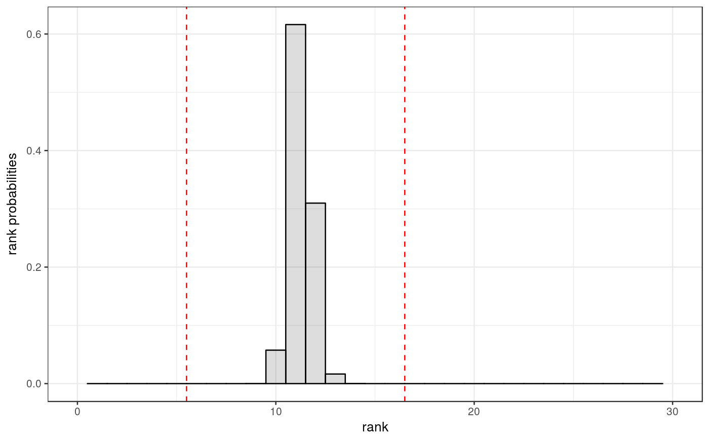
The output of SDP_rnk_pred is a is a list of three elements:

• P: the estimated probability vector (in form of a tibble to avoid confusion about the index),

• bnds: the Pataki bounds,

• plot: a histogram plot (ggplot2) of the probability vector (the vertical lines indicate the Pataki bounds).

Details

The semidefinite program is assumed to be of the form $$\underset{X\in\mathcal{S}^n}{\text{min}} \quad \langle C,X\rangle_{\mathcal{S}^n}$$ $$\text{subject to} \quad \langle A_k,X\rangle_{\mathcal{S}^n}=b_k ,\quad k=1,\ldots,m$$ $$X\succeq 0.$$ Generically, if a solution to this program exists, then it is unique, and its rank satisfies some inequalities, known as Pataki Inequalities. In the natural random model the rank probabilities can be expressed in terms of curvature measures, which is what this function estimates. See the vignette accompanying the symconivol package for more details and references.

See also

Package: symconivol

Examples

library(tidyverse)
#> ── Attaching packages ─────────────────────────────────────── tidyverse 1.2.1 ──
#> ✔ ggplot2 2.2.1     ✔ purrr   0.2.4
#> ✔ tibble  1.4.2     ✔ dplyr   0.7.4
#> ✔ tidyr   0.7.2     ✔ stringr 1.3.0
#> ✔ readr   1.1.1     ✔ forcats 0.2.0
#> ── Conflicts ────────────────────────────────────────── tidyverse_conflicts() ──
#> ✖ dplyr::filter() masks stats::filter()
#> ✖ dplyr::lag()    masks stats::lag()
SP <- SDP_rnk_pred(30,150)

print(SP$P)
#> # A tibble: 31 x 2
#>     `k=` `Prob(rk_sol=k)=`
#>    <int>             <dbl>
#>  1     0          0.      
#>  2     1          0.      
#>  3     2          0.      
#>  4     3          0.      
#>  5     4          0.      
#>  6     5          0.      
#>  7     6          9.45e-33
#>  8     7          7.99e-19
#>  9     8          4.09e-10
#> 10     9          9.50e- 5
#> # ... with 21 more rows
print(SP$bnds)
#> [1]  6 16
print(SP$plot)