Stan model creation for Bayesian posterior given direct samples, enforcing log-concavity
polyh_stan generates inputs for Stan (data list and model string or external file)
for sampling from the posterior distribution,
given direct (multinomial) samples of the intrinsic volumes distribution.
polyh_stan(multsamp, dimC, linC, prior = "noninformative", v_prior = NA,
  filename = NA, overwrite = FALSE)
Arguments
| multsamp | vector of integers representing a sample from the multinomial intrinsic volumes distribution of a convex cone |
|---|---|
| dimC | the dimension of the cone |
| linC | the lineality of the cone |
| prior | either "noninformative" (default) or "informative" |
| v_prior | a prior estimate of the vector of intrinsic volumes (NA by default) |
| filename | filename for output (NA by default, in which case the return is a string) |
| overwrite | logical; determines whether the output should overwrite an existing file |
Value
If filename==NA then the output of polyh_stan is a list containing the following elements:
model: a string that forms the description of the Stan model,data: a data list containing the prepared data to be used for defining a Stan model object, ## rest still has to be adapted ##variable.names: the single string "V" to be used as additional parameter when creating samples from the JAGS object to indicate that only this vector should be tracked.
If filename!=NA then the model string will be written to the file with
the specified name and the output will only contain the elements data
and variable.names.
Details
The prior distribution is taken on the log-concavity parameters (second iterated differences of the logarithms of the intrinsic volumes), which enforces log-concavity of the intrinsic volumes.
Note
See this vignette for further info.
See also
polyh_rivols_gen, polyh_rivols_ineq,
polyh_bayes
Package: conivol
Examples
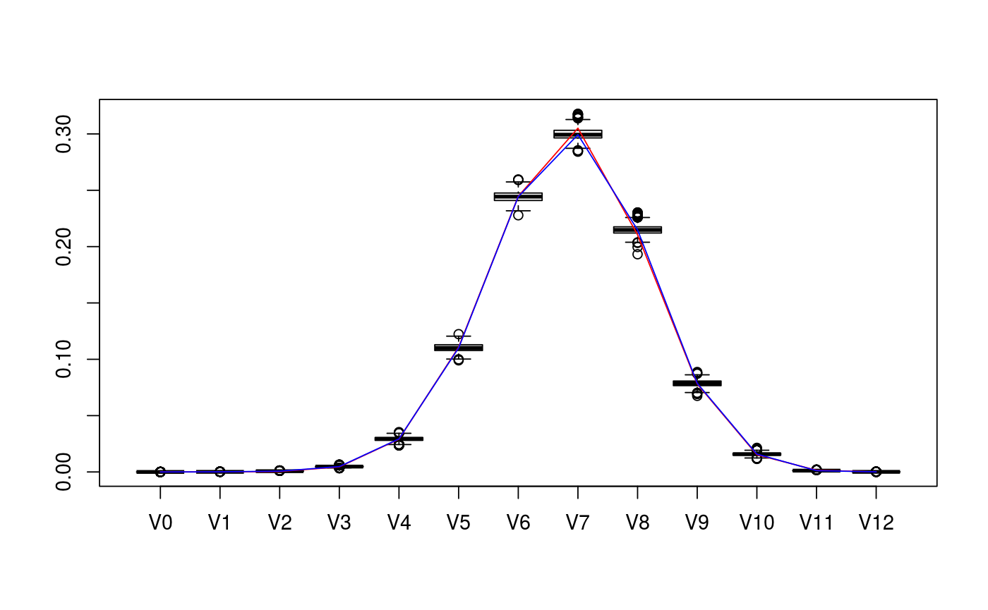
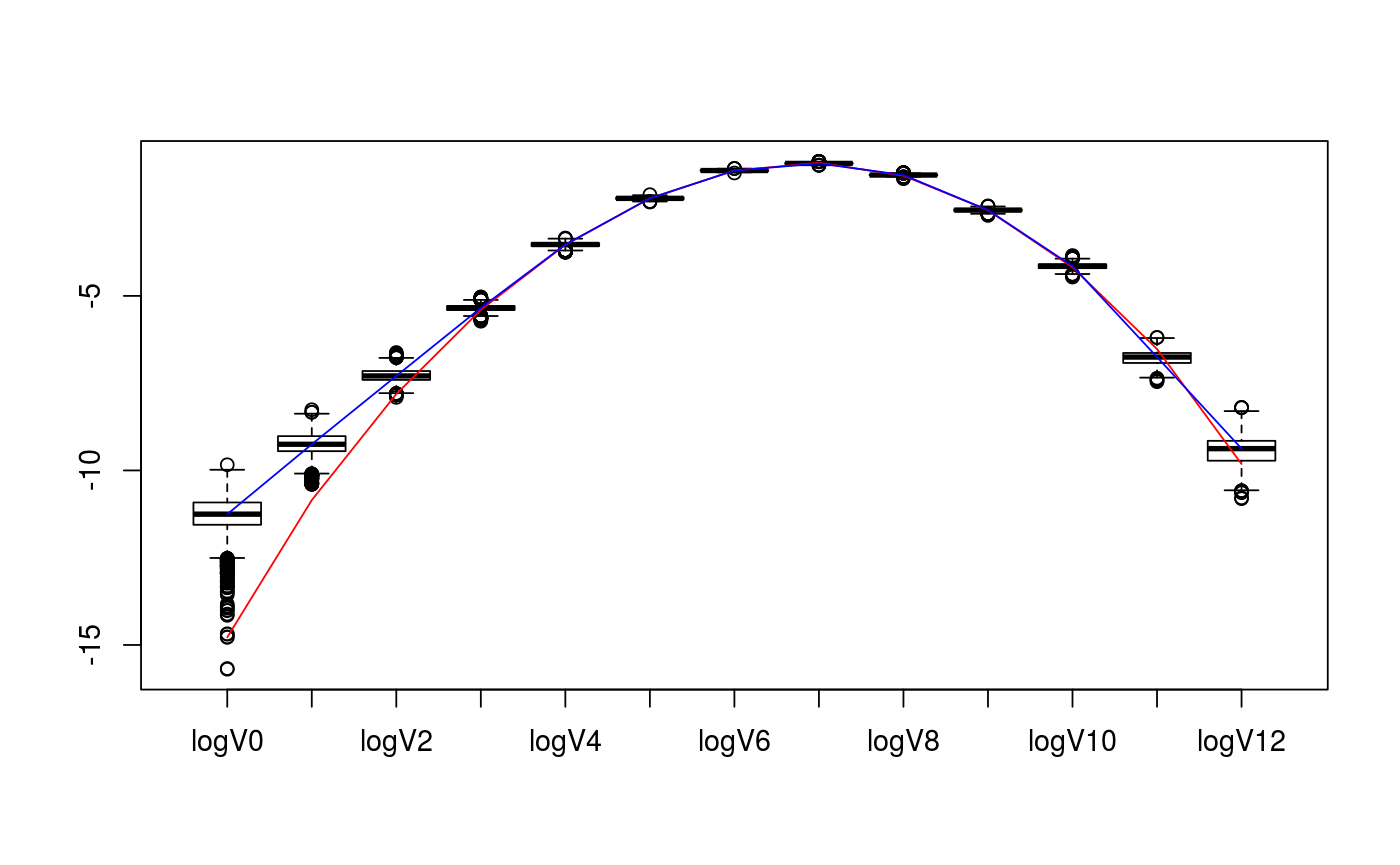
library(rstan)#>#>#>#> #> #># set parameters of cones D <- c(5,7) cone_types <- c("BC","BCp") d <- sum(D) # collect matrix representation and true intrinsic volumes v <- weyl_ivols(D, cone_types, product = TRUE) A <- weyl_matrix(D, cone_types, product = TRUE) true_data <- list( ivols=v, A=A ) print(true_data)#> $ivols #> [1] 3.814697e-07 1.937382e-05 4.049618e-04 4.514140e-03 2.911474e-02 #> [6] 1.107105e-01 2.446381e-01 3.051200e-01 2.105028e-01 7.816557e-02 #> [11] 1.528444e-02 1.470407e-03 5.455017e-05 #> #> $A #> [,1] [,2] [,3] [,4] [,5] [,6] [,7] [,8] [,9] [,10] [,11] [,12] #> [1,] -1 1 0 0 0 0 0 0 0 0 0 0 #> [2,] 0 -1 1 0 0 0 0 0 0 0 0 0 #> [3,] 0 0 -1 1 0 0 0 0 0 0 0 0 #> [4,] 0 0 0 -1 1 0 0 0 0 0 0 0 #> [5,] 0 0 0 0 -1 0 0 0 0 0 0 0 #> [6,] 0 0 0 0 0 1 0 0 0 0 0 0 #> [7,] 0 0 0 0 0 1 1 0 0 0 0 0 #> [8,] 0 0 0 0 0 1 1 1 0 0 0 0 #> [9,] 0 0 0 0 0 1 1 1 1 0 0 0 #> [10,] 0 0 0 0 0 1 1 1 1 1 0 0 #> [11,] 0 0 0 0 0 1 1 1 1 1 1 0 #> [12,] 0 0 0 0 0 1 1 1 1 1 1 1 #># collect sample data from intrinsic volumes distribution n <- 10^4 set.seed(1234) out <- polyh_rivols_ineq(n,A) str(out)#> List of 7 #> $ dimC : int 12 #> $ linC : int 0 #> $ QL : logi NA #> $ QC : num [1:12, 1:12] 1 0 0 0 0 0 0 0 0 0 ... #> $ A_reduced: num [1:12, 1:12] -1 0 0 0 0 0 0 0 0 0 ... #> $ samples : int [1:10000] 8 7 7 8 6 6 8 6 9 4 ... #> $ multsamp : int [1:13] 0 0 6 53 294 1093 2445 3002 2156 782 ...# define Stan model filename <- "ex_stan_model.stan" staninp <- polyh_stan(out$multsamp, out$dimC, out$linC, prior="informative", filename=filename) # run the Stan model sink("no-output.txt") stanfit <- stan( file = filename, data = staninp$data, chains = 4, warmup = 1000, iter = 2000, cores = 2, refresh = 200 )#> In file included from /home/damlunx/R/x86_64-pc-linux-gnu-library/3.4/BH/include/boost/config.hpp:39:0, #> from /home/damlunx/R/x86_64-pc-linux-gnu-library/3.4/BH/include/boost/math/tools/config.hpp:13, #> from /home/damlunx/R/x86_64-pc-linux-gnu-library/3.4/StanHeaders/include/stan/math/rev/core/var.hpp:7, #> from /home/damlunx/R/x86_64-pc-linux-gnu-library/3.4/StanHeaders/include/stan/math/rev/core/gevv_vvv_vari.hpp:5, #> from /home/damlunx/R/x86_64-pc-linux-gnu-library/3.4/StanHeaders/include/stan/math/rev/core.hpp:12, #> from /home/damlunx/R/x86_64-pc-linux-gnu-library/3.4/StanHeaders/include/stan/math/rev/mat.hpp:4, #> from /home/damlunx/R/x86_64-pc-linux-gnu-library/3.4/StanHeaders/include/stan/math.hpp:4, #> from /home/damlunx/R/x86_64-pc-linux-gnu-library/3.4/StanHeaders/include/src/stan/model/model_header.hpp:4, #> from file583a47333750.cpp:8: #> /home/damlunx/R/x86_64-pc-linux-gnu-library/3.4/BH/include/boost/config/compiler/gcc.hpp:186:0: warning: "BOOST_NO_CXX11_RVALUE_REFERENCES" redefined #> # define BOOST_NO_CXX11_RVALUE_REFERENCES #> ^ #> <command-line>:0:0: note: this is the location of the previous definition #> cc1plus: warning: unrecognized command line option ‘-Wno-macro-redefined’#> Warning: There were 1016 divergent transitions after warmup. Increasing adapt_delta above 0.8 may help. See #> http://mc-stan.org/misc/warnings.html#divergent-transitions-after-warmup#> Warning: Examine the pairs() plot to diagnose sampling problemssink() file.remove("no-output.txt")#> [1] TRUE#> List of 5 #> $ t : num [1:4000, 1:13] 1.07e-11 2.95e-07 3.34e-02 2.47e-16 4.35e-15 ... #> ..- attr(*, "dimnames")=List of 2 #> .. ..$ iterations: NULL #> .. ..$ : NULL #> $ v_nonz : num [1:4000, 1:13] 0.00236 0.00407 0.00394 0.00275 0.0026 ... #> ..- attr(*, "dimnames")=List of 2 #> .. ..$ iterations: NULL #> .. ..$ : NULL #> $ V : num [1:4000, 1:13] 8.46e-06 1.73e-05 1.73e-05 1.10e-05 1.03e-05 ... #> ..- attr(*, "dimnames")=List of 2 #> .. ..$ iterations: NULL #> .. ..$ : NULL #> $ logV_nonz: num [1:4000, 1:13] -11.7 -11 -11 -11.4 -11.5 ... #> ..- attr(*, "dimnames")=List of 2 #> .. ..$ iterations: NULL #> .. ..$ : NULL #> $ lp__ : num [1:4000(1d)] -16881 -16881 -16884 -16885 -16886 ... #> ..- attr(*, "dimnames")=List of 1 #> .. ..$ iterations: NULL# remove Stan file file.remove(filename)#> [1] TRUE# compare posterior median with true values v_est_med <- apply(extract(stanfit)$V, 2, FUN = median) v_est_med / v#> [1] 33.9626993 4.9564095 1.6796997 1.0582269 1.0080429 0.9945965 #> [7] 0.9987856 0.9811167 1.0204250 1.0066855 1.0342103 0.7938889 #> [13] 1.5538762sum( (v_est_med-v)^2 )#> [1] 5.297396e-05# display boxplot of posterior distribution, overlayed with true values data <- as.data.frame( extract(stanfit)$V ) colnames(data) <- paste0(rep("V",d+1),as.character(0:d)) boxplot( value~key, tidyr::gather( data, factor_key=TRUE ) )lines(1+0:d, v, col="red")lines(1+0:d, v_est_med, col="blue")# display boxplot of posterior distribution of logs, overlayed with true values data <- as.data.frame( extract(stanfit)$logV_nonz ) colnames(data) <- paste0(rep("logV",d+1),as.character(0:d)) boxplot( value~key, tidyr::gather( data, factor_key=TRUE ) )lines(1+0:d, log(v), col="red")lines(1+0:d, log(v_est_med), col="blue")