Finding the weights of the bivariate chi-bar-squared distribution using EM algorithm

estim_em produces EM-type iterates from a two-column matrix whose rows form iid samples from a bivariate chi-bar-squared distribution.

estim_em(d, m_samp, N = 20, v_init = NULL, init_mode = 0, lambda = 0,
  no_of_lcc_projections = 1, lcc_amount = 0, extrapolate = 0,
  selfdual = FALSE, data = NULL)

Arguments

d	the dimension of the bivariate chi-bar squared distribution.
m_samp	two-column matrix whose rows from iid samples from a bivariate chi-bar-squared distribution.
N	the number of iterates that shall be produced.
v_init	the starting point for the EM iterates; if none are provided, the starting point is found in a way specified by the input init_mode.
init_mode	specifies the way through which the initial estimate is found: init_mode==0: uniform distribution init_mode==1: discretized normal distribution init_mode==2: circular cone fitting statdim init_mode==3: circular cone fitting variance init_mode==4: circular cone fitting statdim and variance (geometric mean) The starting point will be returned as the first row in the output matrix.
lambda	nonnegative parameters which, if positive, enforce the log-concavity inequalities. Enforcing these may have negative effects on the performance. lambda can be a scalar or vector of length d-1.
no_of_lcc_projections	number of projections on the log-concavity cone
lcc_amount	constant for strict log-concavity
extrapolate	specifies the way the edge cases are handled: extrapolate==0: extrapolate v_d if no x in C and extrapolate v_0 if no x in C° extrapolate==1: extrapolate v_d, do not extrapolate v_0 extrapolate==2: extrapolate v_0, do not extrapolate v_d extrapolate==3: extrapolate v_0 and v_d extrapolate<0: neither extrapolate v_0 nor v_d
selfdual	logical; if TRUE, the symmetry equations v[k+1]==v[d-k+1], with k=0,...,d, are enforced. These equations hold for the intrinsic volumes of self-dual cones.
data	output of prepare_em(d, m_samp); this can be called outside and passed as input to avoid re-executing this potentially time-consuming step.

Value

The output of estim_em is a list of an (N+1)-by-(d+1) matrix whose rows constitute EM-type iterates, which may or may not converge to the maximum likelihood estimate of the mixing weights of the bivariate chi-bar-squared distribution, and the corresponding values of the log-likelihood function.

Details

The sequence of iterates may or may not converge to the maximum likelihood estimate of the mixing weights of the distribution. Log-concavity of the intrinsic volumes is enforced by projecting the logarithms onto the cone of log-concave sequences; this can be turned off by setting no_of_lcc_projections=0.

See also

rbichibarsq, circ_rbichibarsq, rbichibarsq_polyh, prepare_em, init_ivols, loglike_ivols

Package: conivol

Examples

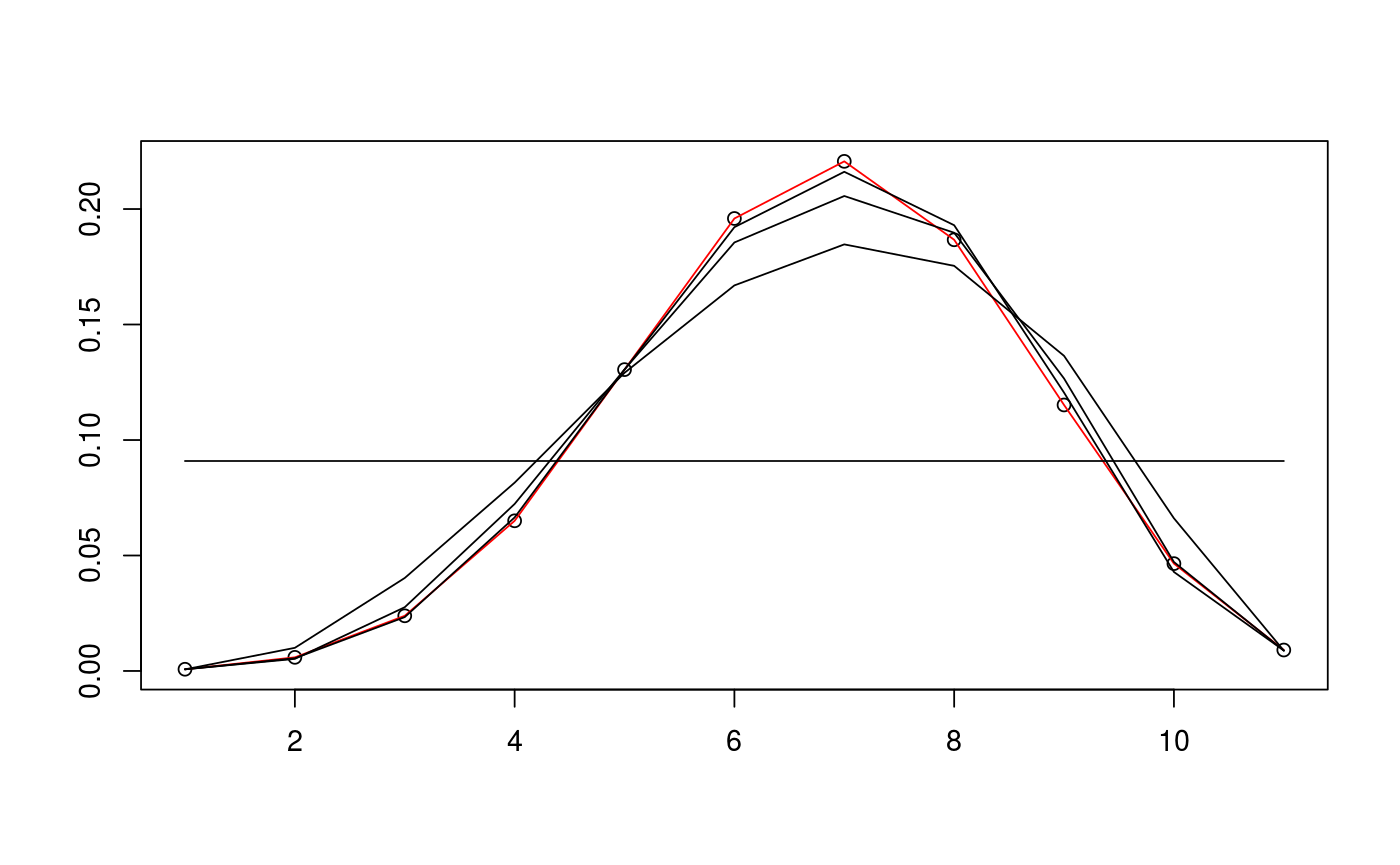
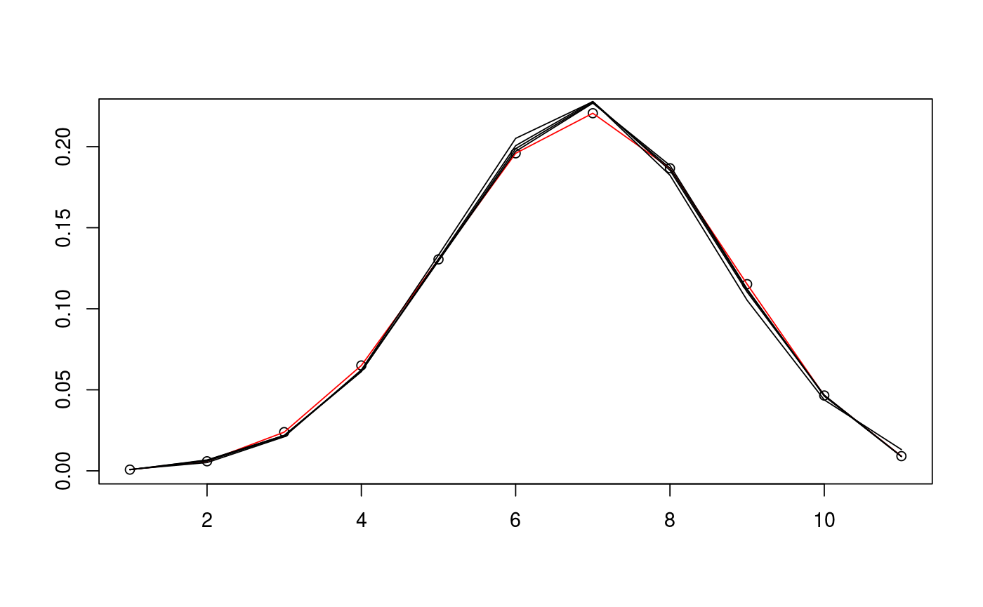
# define cone and find sample data
D <- c(5,5)
alpha <- c(pi/3,pi/4)
d <- sum(D)
N <- 10^5
v_exact <- circ_ivols( D, alpha, product=TRUE )
m_samp <- rbichibarsq(N,v_exact)

# prepare data and run EM algorithm twice with different inits
data <- prepare_em( d, m_samp )
est1 <- estim_em( d, m_samp, data=data )
est2 <- estim_em( d, m_samp, init_mode=1, data=data )

# plot the iterates of the first EM run
plot(1+0:d, v_exact, ann=FALSE)
lines(1+0:d, v_exact, col="red")
lines(1+0:d, est1$iterates[1,])
lines(1+0:d, est1$iterates[5,])
lines(1+0:d, est1$iterates[10,])
lines(1+0:d, est1$iterates[21,])

# plot the iterates of the second EM run
plot(1+0:d, v_exact, ann=FALSE)
lines(1+0:d, v_exact, col="red")
lines(1+0:d, est2$iterates[1,])
lines(1+0:d, est2$iterates[5,])
lines(1+0:d, est2$iterates[10,])
lines(1+0:d, est2$iterates[21,])